
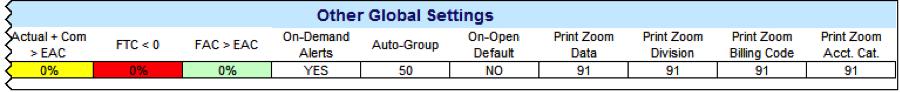
Other Global Settings affect all modes of the BFA workbook.
Division Subtotals

The Division Totals worksheet is created when you select the Division Totals command on the Spitfire menu. You can modify the color and content of the subtotal rows through the Division Subtotal setting.
To set a color for your subtotal rows:
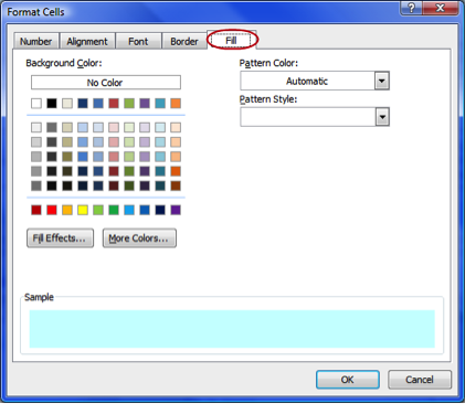
- On the Setup worksheet, in the Division Subtotal cell, right-click and select Format Cells.
- From the Fill tab, select your color.

- Click OK.
Note: The color change will take effect the next time you choose the Division Totals option on your Data Worksheet.
Changing the Content Format
The Content of the cell determines the start location and the length of the characters to be used for creating the Division subtotals.
The first digit signifies where the first “significant” subtotal digit (your division code) is found. For example, if your cost codes are standard CSI codes, then 1 digit would be the significant digit since that is where your CSI division code begins.
The second digit represents the number of digits to use when creating a subtotal group (how many digits in your division code). For example, if your cost codes have five digits (ex: 02350, 03250, 03100, etc), an entry of 2 will group your cost codes by two digits.
For example, if you use 1,2 in the Division Subtotal cell, and if your BFA worksheet uses the CSI Codes (02350, 03250, 03100, etc), your subtotals would use the first digit (first digit = 1) as the starting point and two (second entry = 2) digits as the count of characters to evaluate and subtotal on 02 and 03.
Subtotal rows are created for each subtotal group and placed on the Division Totals worksheet. Subtotals are calculated for a group’s constituent rows for each column that has a page total.
To change the content format for subtotals:
- Click the Division Subtotal cell.
- Type a digit to signify which position begins the significant portion of your Cost Code for subtotaling purposes, type a comma, then type a digit to signify the number of significant characters to be used in your subtotal.
Freeze Clm
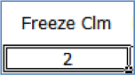
This setting indicates how many Data worksheet columns should be frozen when you scroll to the right.
To change the number of columns to be frozen, type the number of columns you want frozen in the Freeze Clm cell. For example, typing 2 means the first two columns (A and B) will be frozen.
Budget Default

This setting provides the default used when entering manual changes to BFA in Budget mode. (For more information, see the Budgets and Period Distribution Focus Guide.) Possible selections are A, which means “add to the existing Budget amount” or R which means “replace the existing Budget amount”. The change type appears on the Manual Budget Change Type column when an amount is entered in the Manual Budget Change mount column (when the BFA workbook is opened from a Budget document).
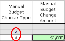
To change your default Manual Change Type option, select A or R from the drop-down menu in the Budget Default cell.
Forecast Default
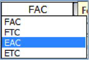
You can choose to set your default Forecast option to FAC (Forecast At Completion) or FTC (Forecast To Completion). If you call your forecasts “estimates,” you can choose EAC or ETC instead. In the worksheet you can use either method as you move from Cost Code to Cost Code or Account Category to Account Category, but your setting here will be the default value.
To set your default Forecast option, select your default from the drop-down menu in the Forecast cell.
Amounts
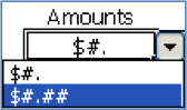
You can change whether numbers will appear as whole numbers ($#) or with two decimal places ($#.##).
To change your default Amounts, select your format choice from the drop-down menu in the Amounts cell.
Display Units
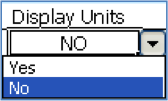
The Display Units option is a convenient way to show (Yes) or hide (No) all unit-related columns at once. The Display Units option also affects if the Forecast Data Entry form is presented with units or not.
To select the Display Units option, select your choice from the drop-down menu in the Display Units cell.
Note: If your Local preferences have specifically hidden any units columns, the “Display Units” option will respect these selections.
Gain/Loss
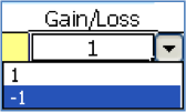
You can indicate whether amounts in gain/loss columns should appear as positive (1) or negative (-1) numbers. This setting also changes the gain/loss columns in the Forecast Data Entry form.
To set how losses appear in gain/loss columns, select your choice from the drop-down menu in the Gain/Loss cell.
Posted and Interim
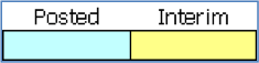
You can set the color of Posted Items to be different from the Spitfire or Site default color by selecting a color for the Posted cell. You can also select the color of Interim items.
Note: Although the new color will not be applied to existing Interim changes already displayed in the Data worksheet, new Interim changes will use the new color. If Local Settings are saved, then reopening the BFA workbook will have the new color selection applied. If multiple users are making interim changes or if you want to keep new changes visually separate from existing interim changes, you can change the interim color (without saving preferences). All changes from this point on will inherit the new color. You can repeat this multiple times as long as the workbook remains open. When closed and reopened, all interim changes will be in one color.
To set a color for your Posted and Interim rows:
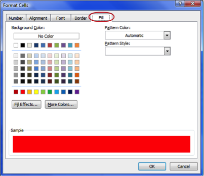
- In the Posted or Interim cell, right-click and select Format Cells.
- From the Fill tab, select your color.
- Click OK.
This color will appear the next time you open the BFA workbook.
Alert Indicators
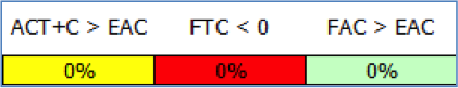
Spitfire includes three default Alert Indicators:
- When Actual Costs plus Committed Costs are greater than the Estimate-At-Completion (ACT + C > EAC).
- When Forecast-to-Complete is less than the Actual Costs plus the Committed Costs (FTC < 0).
- When Forecast-At-Completion is greater than the Estimate-At-Completion (FAC > EAC).
Each Alert Indicator allows you to set the alert’s color and tolerance level.
Setting the Color
To set the color for your Alert Indicators:
- In the FTC < 0, ACT + C > EAC, or FAC > EAC cell, right-click and select Format Cells.
- From the Fill tab, select your color.
- Click OK.
Setting the Tolerance Level
If the tolerance level is set to 0%, the alert is turned off. If the tolerance alert is set to 1% or greater, the alert is turned on.
Note: 1% tolerance allows for rounding exclusions where the amounts are a few pennies and not worth reporting.
To set a tolerance level for your Alert Indicators, type the desired tolerance level in the Alert Indicator cell.
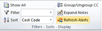
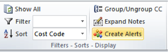
On-Demand Alerts

By default the Alerts are created automatically (No). You can choose to create Alerts manually (Yes). If you choose Yes (and have Alerts set up), a new option will appear on the Spitfire BFA ribbon when you go back to the Data worksheet. Use the Create Alerts option (or the Refresh Alerts option) when you want to create Alerts on demand.
To select the On-Demand Alerts option, select your choice from the drop-down menu in the On-Demand Alerts cell.
Auto-Group
The grouping and expand/collapse features of Account Categories within Cost Codes requires significant Microsoft Excel overhead, determined by the number of Cost Codes. If the grouping process significantly impedes the ability to navigate the worksheet and it is more convenient to not group the Cost Codes, you can change this setting to reduce the impact of Auto-Grouping. The entry identifies the number of Cost Codes rows above which Auto-Grouping is turned off. Functions that require a grouped structure ignore this setting.
To set the Auto-Group number, type the number rows which should allow grouping, in the Auto-Group cell. Rows above this number will not be grouped.
On-Open Default
You can choose to open the Data worksheet in expanded view, where the Account Categories are visible within the Cost Codes (Yes) or to open the Data worksheet with the Cost Codes contracted (No). For this option to have effect, the Auto-Group count must exceed the Cost Code count.
To select the On-Open Default option, select your choice from the drop-down menu in the On-Open Default cell.
Print Zoom Data

The worksheet page print area is automatically adjusted to include all visible rows and columns; therefore column visibility and filters impact the print area. The Print Zoom Data feature provides you with some control to format the Data worksheet’s printed output to fit a specific size.
You can set the print size as a percentage of the original size (100%). You must enter a value between 10% and 400%.
To set the print zoom level, enter a print percentage in the Print Zoom cell.
Print Zoom Division

The Print Zoom Division feature provides you with some control to format the Division worksheet’s printed output to fit a specific size.
You can set the print size, used when the worksheet is printed, as a percentage of the original (100%). You must enter a value between 10 and 400.
To set the print zoom level, enter a print percentage in the Print Zoom cell.
Print Zoom Billing Code
The Print Zoom Billing Code feature provides you with some control to format the Billing Code worksheet’s printed output to fit a specific size.
You can set the print size, used when the worksheet is printed, as a percentage of the original (100%). You must enter a value between 10 and 400.
To set the print zoom level, enter a print percentage in the Print Zoom cell.
Print Zoom Acct. Cat.
The Print Zoom Acct. Cat. feature provides you with some control to format the Account Category worksheet’s printed output to fit a specific size.
You can set the print size, used when the worksheet is printed, as a percentage of the original (100%). You must enter a value between 10 and 400.
To set the print zoom level, type the desired print percentage in the Print Zoom cell.