To indicate a code for a User Calc Field column:
- Scroll to a User Calc Field column.
- On row 67, select a code from the drop-down to indicate how you want subtotals to be handled on your Division Totals or Billing Code Totals worksheet.
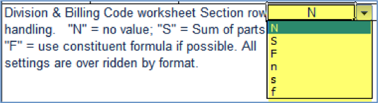
- F – use the formula indicated for the column (in row 61) converted to the appropriate worksheet (Division Totals or Billing Codes), possibly using ratios.
- N – no value; leave the cell blank. This option is used by Spitfire whenever the resulting value created by a sum or formula is nonsensical (such as when adding units with different units of measure).
- S – use the sum of the constituent amounts. This option is often used for money.
User Save Text Columns (Site)
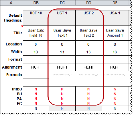
If you scroll to the right on the Setup worksheet, you will find two possible user-defined text columns (initially called UST 1 and UST 2). These columns can hold text not elsewhere on the Data worksheet. You can change the title, location, width, and alignment of these columns as described previously.
User Save Amounts Columns (Site)
If you scroll to the right on the Setup worksheet, you will find three possible user-defined amount columns (initially called USA 1 through USA 3). These columns can hold numeric amounts not elsewhere on the Data worksheet. You can change the title, location, width and alignment of these columns as described previously.
Subtotal Row Handling
If you want to use any of the User Save Amount columns in your Division Totals or Billing Code Totals worksheet, you should indicate how subtotal rows are to be handled on those columns – whether the subtotal row should sum its constituent amounts, should use a formula, or should remain blank.
During the initial creation of the Division Totals or Billing Code Totals worksheet, User Save Amounts are reviewed and converted for use in the associated worksheet. The conversion remains in place during the session of BFA or until the user makes changes to the Setup data. If a formula would return invalid results, that User Save Amount column is treated as N for none (blank).
To indicate a code for a User Save Amount column:
- Scroll to a User Save Account column.
- On row 67, select a code from the drop-down menu to indicate how you want subtotals to be handled on your Division Totals or Billing Code Totals worksheet.
- F – use the formula indicated for the column (in row 61) converted to the appropriate worksheet (Division Totals or Billing Codes), possibly using ratios.
- N – no value; leave the cell blank. This option is used by Spitfire whenever the resulting value created by a sum or formula is nonsensical (such as when adding units with different units of measure).
- S – use the sum of the constituent amounts. This option is often used for money.
Forward Looking Rows
You can indicate how many blank rows the Import Wizard should take into consideration when importing data from an import worksheet. This allows the import worksheet to have blank rows between data rows.
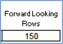
To set the number of forward-looking rows, type the number of rows that the Import Wizard should skip over when looking for data In the Forward Looking Rows cell (column V).
Alerts
You can modify one, two, or three of the Spitfire-default Alert triggers. You can change the title of each Alert, as well as conditions that will trigger each alert.
The conditions, together with the tolerance level established elsewhere on the Setup worksheet, determine when Alerts are triggered.
Note: Alerts are disabled if either the prime or secondary column is not active (ie, location = 0) in the Data worksheet, regardless of the tolerance level established for the Alert.
To change the title of an Alert, type a new title in the Title column and then leave the cell.
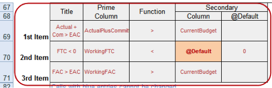
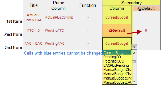
To indicate the conditions to trigger the Alert:
- In the Prime Column cell select your primary data column from the drop-down menu. The data column must be one that contains amounts (not text) within BFA.
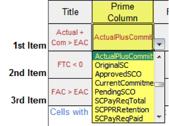
- In the Function cell, select a function from the drop-down menu.
- In the Secondary | Column cell, select a comparison data column from the drop-down or select @Default if you want to enter a constant in the @Default cell.
Note: Tolerance percentages are converted into decimals for calculation purposes (ie: 10% = .10).
Alert Functions
| When Secondary is a data column | When Secondary is a constant | |
|
Trigger Alert If |
||
| < | Prime is less than Secondary
OR (Prime – Secondary) < (Prime * Tolerance) |
Prime * (1 + Tolerance) < Secondary |
| > | Prime is greater than Secondary
OR (Prime – Secondary) > (Prime * (Tolerance * -1)) |
Prime * (1 + Tolerance) > Secondary |
| ≤ | Prime is less than or equal to Secondary
OR (Prime – Secondary) <= (Prime * Tolerance) |
Prime * (1 + Tolerance) < = Secondary |
| ≥ | Prime is greater than or equal to Secondary
OR (Prime – Secondary) >= (Prime * (Tolerance * -1)) |
Prime * (1 + Tolerance) >= Secondary |
| / | Prime divided by Secondary is greater than Tolerance | |
| + | Prime equals the Secondary
Note: Although this calculation does not use Tolerance, a tolerance level other than 0 is needed to activate the Alert. |
|
Filters
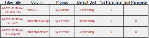
You can modify up to three Spitfire-default Filters (Above or Below $ Gain/Loss, Above or Below % Spent, and Above or Below % Complete). You can re-label each filter, as well as select the column on which to filter, and set the default sort direction and default amounts/percentages.
To modify a Filter:
- In the Filter Title cell, enter a descriptive title for your filter.
- In the Column cell, select the column on which you want to filter, from the drop-down menu. Only data columns with amounts or percentages are valid choices.

The data column you select will determine if the Prompt cell indicates By Amount or By Percent. If the data column you select is a User-Calc column, however, you can indicate if the Prompt should be By Amount or By Percent. - In the Default Sort cell, select a direction from the drop-down menu.
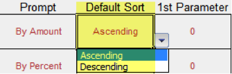
- In the 1st Parameter cell, type the default number that should appear in the first parameter field.
- If appropriate, in the 2nd Parameter cell, type the default number that should appear in the second parameter field.
Sorts
You can modify up to three Spitfire-defaut Sorts: Gain/Loss, % Spent, % Complete.
To modify a Sort:
- In Sort Title, enter a descriptive title for your sort. You can also keep the title given and just modify the remaining columns.
- In Column, select the column you want to sort from the drop-down menu.
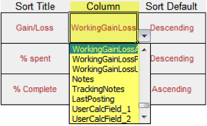
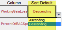
- In Sort Default, select a direction from the drop-down menu.
Executive Overview
These site settings control the contents of the two charts on the Executive Overview worksheet. You can change the title of each chart as well as change the data used for the columns in the charts.
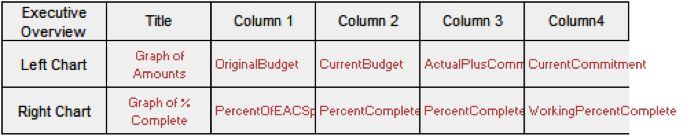
To modify a chart:
- In Title enter a descriptive title for your chart.
- In each of the Column cells, select the data you want to use from the drop-down menu.
