KBA-01545: Executive Dashboard Custom Formulas in Supplemental Workbooks.

Question:

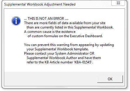
I received the ‘Supplemental Workbook Adjustment Needed‘ message shown below.  What should I do?

Answer:

You need to add the Executive Dashboard (EDB) Supplemental Workbook (SW) fields that are missing in the Column Selection drop-down list on your Setup worksheet.

Background:

When the EDB SW opens, embedded code compares each data field within the workbook to those data fields being passed in from the ‘EDB-filtered data set‘.  When a mismatch occurs, the above message is displayed. The mismatch is most often a result of site configurations, specifically the addition of custom calculation formulas that create new data elements in the EDB results set.  While the new fields may not be required within a properly functioning SW, it is best to synchronize the data fields between the SW and the EDB-filtered data set.

Changes to a SW Report Creation template require manual input and cannot be automated.  These changes should be completed by the site System Administrator or the site Supplemental Workbook author.

Spitfire recommends the use of two active workbook sessions of Microsoft Excel to minimize possible keyboard, naming and saving errors when making these changes.  The following steps assume two workbooks opened at the same time.

To synchronize the data fields:

Note: You will need to have System Admin rights.  If your SW is not in the Spitfire template library, start with step 2.

1. Download the appropriate Exec Dashboard Export template from the Templates tool.  (For more information, see the Focus on the Manage Dashboard guide.)
2. From your desktop (or file location if your SW was not in your template library to begin with), highlight the icon for the downloaded template file and right-click.
3. Select Open. This will launch Microsoft Excel and open the workbook as a template, allowing you to save changes to the template.  An Open in Template mode message should appear.  We refer to this workbook as workbook 1 for the rest of these instructions.
4. In this workbook, navigate to the Column Setup worksheet.
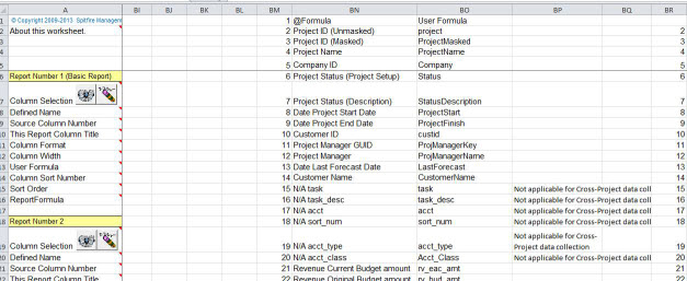
5. Navigate to column BM on row 2.  The range BM2 – BRx represents the data fields within the workbook.
6. Go to the Executive Dashboard in sfPMS, enter filter criteria and refresh.
7. Use the export icon and select the same template as the one you downloaded.  This will create a second session of Microsoft Excel.  We will refer to this workbook as workbook 2 for the rest of these instructions.
8. In workbook 2, navigate to the Column Setup worksheet.
   Note: if the Column Setup worksheet is not visible, you need to unhide it: Select any worksheet tab, right-click and select Column Setup in the Unhide box.
9. Highlight all cells containing data from BS2 to BUx and (using the ribbon option or the Ctrt+C keyboard shortcut) copy this group of cells to the clipboard. This range is the EDB filtered data set.
10. Paste the clipboard contents into cell BG2 on the Column Setup worksheet in workbook 1
11. Close workbook 2 without saving and exit this session of Microsoft Excel.  The remaining instructions are for worksheet 1.
12. Carefully compare the names in column BH to the names in column BO.  Disregard the numbers in the corresponding columns for now.
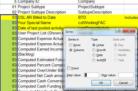
    Note in the example below how cstWorkingFAC appears in column BH but not in column BO.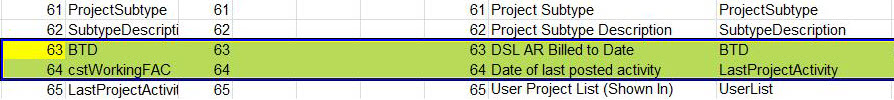
13. Apply the following steps to each missing element until the contents in column BH and column BO match, always adjusting the columns BM to BR.  We will refer to each row as the Missing Element Row.
    1. Select the cells in columns BM to BR on the Missing Element Row.
    2. With the group selected, right-click and select Insert from the pop-up menu.  Select Shift Cells Down when prompted.
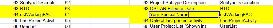
    3. Copy the element Name from column BH to column BO on the Missing Element Row.
    4. Type the reference name in column BN on the Missing Element Row.  This reference name will display in the Column Selection drop-down list.
       
14. Locate and select the group of cells you pasted in step 10, starting with BG2 to BI2.
15. Using the ribbon option to clear all or the keyboard shortcut to delete, remove the unwanted content in these columns.
16. Create a sequential numbering pattern in columns BM and BR.
    1. Starting at the first correction point or the top of the list, highlight all the cells in the appropriate column with content in the adjacent columns going down to the bottom of the list.
    2. Right-click to bring up the Series pop-up window and click OK for the defaults (Column, Linear, Step Value=1). The results should be that BM and BR are sequential and match to the end of the list.  Verify also that there are no blanks in column BN or BO.
17. Note the Excel row number containing the last item of the list.
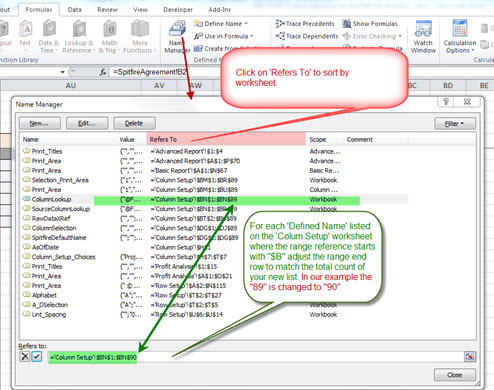
18. Select Name Manager from the Formula ribbon.
19. Click on the column header Refers To to sort the Defined Names by worksheet.
20. For each Defined Name with a reference to the Column Setup worksheet with a reference that begins with $B (=‘Column Setup‘!$B#S#:$B#$##) adjust the range end row to match the Excel row containing the last member of the list.
21. Once all references are adjusted, close the Name Manager and save your work.
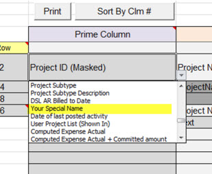
22. Navigate to any of the Select Column cells and review the list.  Each of your new reference names should appear in the list and in order.
    
23. Navigate to cell A1 on this worksheet and on the Spitfire Agreement worksheet.
24. Save and exit this workbook.
25. Back at the Template tool, upload the revised template and save.  The Supplemental Workbook Adjustment Needed message should not appear the next time you use this template.

KBA-01545; Last updated: October 14, 2016 at 10:27 am